Writing binary by hand

2022-09-24 | Martin Hoppenheit | 27 min read

This post is based on a talk I gave at iPres 2022 (slides). It explains how to read a file format specification (in this example, TIFF) and based on that build a minimal binary file by hand.

The file we are going to build will look rather boring, but that’s not the point because we are not so much interested in the image content but in the file structure. (Note that the image shown here is not a TIFF but a PNG file because that’s easier to display in most web browsers. The TIFF file is here.)

Why?

First off, why would anyone want to build binary files by hand? For me, the most important reason is learning about file formats. When I really want to know how a file format is structured, where and in which form it stores its payload and metadata, in which parts it is robust or fragile, where it has ambiguous edge cases, … then reading the file format specification alone is not enough. I want to build something from scratch then, play around, try out different variants, intentionally break (and fix) things. Here is a bunch of example files I built for that purpose. Apart from that, creating binary files by hand can be useful for all kinds of documentation like describing issues (example, another example), or to create test data for file format-related tools like JHOVE (example).

How?

The most general tool when working with binary files is a hex editor which displays binary data as a sequence of hex characters. (Look here if you need a primer or refreshment on binary/hex notation.) A hex editor is quite versatile and can be used to view, edit, and write files on the binary level. You could absolutely use one to follow along this tutorial. However, since it looks like this …

00000000: 4d4d 002a 0000 0008 0008 0100 0003 0000  MM.*............
00000010: 0001 0200 0000 0101 0003 0000 0001 0140  ...............@
00000020: 0000 0106 0003 0000 0001 0000 0000 0111  ................
00000030: 0003 0000 0003 0000 006e 0116 0003 0000  .........n......
00000040: 0001 0080 0000 0117 0003 0000 0003 0000  ................
00000050: 0074 011a 0005 0000 0001 0000 007a 011b  .t...........z..
00000060: 0005 0000 0001 0000 0082 0000 0000 008a  ................
00000070: 208a 408a 2000 2000 1000 0000 012c 0000   .@. . ......,..
00000080: 0001 0000 012c 0000 0001 ffff ffff ffff  .....,..........
00000090: ffff ffff ffff ffff ffff ffff ffff ffff  ................
000000a0: ffff ffff ffff ffff ffff ffff ffff ffff  ................
000000b0: ffff ffff ffff ffff ffff ffff ffff ffff  ................
000000c0: ffff ffff ffff ffff ffff ffff ffff ffff  ................
000000d0: ffff ffff ffff ffff ffff ffff ffff ffff  ................
000000e0: ffff ffff ffff ffff ffff ffff ffff ffff  ................
000000f0: ffff ffff ffff ffff ffff ffff ffff ffff  ................
00000100: ffff ffff ffff ffff ffff ffff ffff ffff  ................
00000110: ffff ffff ffff ffff ffff ffff ffff ffff  ................
00000120: ffff ffff ffff ffff ffff ffff ffff ffff  ................
00000130: ffff ffff ffff ffff ffff ffff ffff ffff  ................

… I would like to propose a different approach: something I call Literate Binary. Literate Binary (a shameless rip-off of Donald Knuth’s Literate Programming) is a combination of Markdown and hex code. The hex code is (mostly) just like the hex code you see in a hex editor, but embedded in human-readable structure and plain text documentation expressed in Markdown, a lightweight markup syntax (think HTML without all those tags). It looks like this:

## Image File Header

Some text explaining what the file header contains.

    4d4d 002a 00000008

Here you see three Markdown elements, which is all you need for this tutorial:

A (second-level) headline, introduced by ## signs.
A regular paragraph, delimited by blank lines.
A so-called code block, indented by four spaces. It contains a sequence of hex characters that represent binary content. Restricting the code block to hex syntax is what makes a Markdown document Literate Binary.

Markdown is widely supported (e.g., it renders nicely on GitHub) and there are many tools (e.g., Pandoc) that convert from Markdown to other document formats like PDF, HTML or Microsoft Word. Further more (and that’s the interesting part), a Literate Binary document can easily be turned into a proper binary file with a tool called lb that takes the hex code from all code blocks in a Markdown file and turns it into a binary. This is how it is used on the command line:

$ lb example.md --output example.tif

Getting started with TIFF

Let’s start by taking a look at the TIFF file format specification (you might want to keep it open in another browser tab since we will be coming back to it all the time).

The first thing I usually do when reading a file format specification is skimming through the table of contents looking for sections called something like “structure”, “overview”, “building blocks” – anything that sounds like either a high level view of the file structure or a definition of the components that make up the file. Parts like this are often good starting points to get a first idea of the general file structure as well as to find references to other sections that serve as a road map through the specification. Another type of content to look out for are sections called “glossary”, “list of …” or “reference guide” because everybody loves a good reference guide, right?

Looking at the TIFF spec’s table of contents you will quickly notice “Section 2: TIFF Structure” on page 13 which sounds like a good start. The second paragraph on that page tells us:

A TIFF file begins with an 8-byte image file header that points to an image file directory (IFD). An image file directory contains information about the image, as well as pointers to the actual image data.

Granted, that does not explain what an image file header or an image file directory is, or how these things look like. But nevertheless, we learn a lot about the top level file structure in this short paragraph: At the beginning of a TIFF file is a component called Image File Header which holds 8 bytes of data. In particular, this data tells us where we should look for another component called Image File Directory (it even has an abbreviation, IFD). The Image File Directory in turn contains “information about the image” (whatever that may be, but probably some kind of metadata) and it points to the main content of the file, the image data. Let’s sketch that out in Markdown, giving each of the mentioned top level components its own section:

# TIFF File Example

## Image File Header

...

## Image File Directory

...

## Image Data

...

Image File Header

What’s next? Still on page 13, we find a description of the Image File Header:

Bytes 0-1: The byte order used within the file. Legal values are “II” (4949.H, little endian) or “MM” (4D4D.H, big endian).

Bytes 2-3: An arbitrary but carefully chosen number (42) that further identifies the file as a TIFF file.

Bytes 4-7: The offset (in bytes) of the first IFD. The directory may be at any location in the file after the header.

So what does that mean? It means the Image File Header consists of three parts.

The first part (the first two bytes of the header; note that counting starts at 0, just like in many programming languages) contains either the hex values 4949 or 4d4d, denoting the byte order used in the file. I don’t want to delve too deep into this topic because it’s a little out of scope here, but let’s just say that byte order or “endianness” defines whether the bytes (not the bits!) in a multi-byte field should be read from left to right or from right to left. This is best explained by an example, for which we use the next part of the Image File Header.

The second part contains the number 42 (because, you know, it’s the answer) which reads 2a in hex. (The conversion from decimal to hexadecimal can be done by hand, by the calculator application on your computer, by one of the many online converters, or by simply entering something like “42 in hex” into your favorite search engine.) Putting this 1-byte number into a 2-byte big endian field results in 002a while putting it into a little endian field results in 2a00. So a big endian TIFF file starts with the bytes 4d4d 002a while a little endian TIFF file starts with the bytes 4949 2a00. The given byte order has to be observed in all numeric multi-byte fields throughout the file.

Finally, the third part contains the offset of the Image File Directory. An offset is simply a position in the file which is determined by counting bytes from the beginning of the file (again, counting starts at 0, so the first byte in a file is always at offset 0). The use of offsets as pointers to locations in a file is not specific to TIFF but very common in binary file formats.

If we decide to use big endian byte order (just my personal preference) and arrange the IFD to start directly after the Image File Header (which means offset 8) we get this:

## Image File Header

Byte order (big endian) + number 42 + offset of first IFD.

    4d4d 002a 00000008

Some trivia before we move on:

The bytes 4949 and 4d4d correspond to the ASCII characters “II” and “MM”, respectively. Think “II” like “Intel” and “MM” like “Motorola”.
With what you have learned about the Image File Header so far you could already design a PRONOM file format identification signature for the TIFF format.

Image File Directory: structure

Moving on to page 14 we learn that

An Image File Directory (IFD) consists of a 2-byte count of the number of directory entries (i.e., the number of fields), followed by a sequence of 12-byte field entries, followed by a 4-byte offset of the next IFD (or 0 if none).

This is followed by a description of the internal structure of an IFD entry:

Bytes 0-1: The Tag that identifies the field.

Bytes 2-3: The field Type.

Bytes 4-7: The number of values (Count) of the indicated Type.

Bytes 8-11: The Value Offset, the file offset (in bytes) of the Value for the field.

Again, that does not tell us what exactly the IFD should contain and it does not explain the meaning of all its components, but it tells us everything we need to know to sketch out the overall structure of the IFD:

## Image File Directory

Number of IFD entries.

    ????

Sequence of IFD entries (tag + type + count + value offset).

    ???? ???? ???????? ????????
    ...

Offset of the next IFD or 0.

    00000000

As you see, we use a placeholder for the number of IFD entries since we don’t know yet how many entries we will need in the end, and also for the sequence of IFD entries. For the last component we simply use 0 because our example file has only one IFD. Multiple IFDs can be used for things like multi-page TIFFs or embedded thumbnails (see also page 16 of the TIFF spec), but in our simple example one IFD is sufficient.

There is some more relevant information on page 15 of the spec but that’s easier to understand with an example, so we will just skip it for now and come back later.

Image File Directory: content

We are now more or less done with Section 2: TIFF Structure, but obviously we don’t have a complete TIFF file yet. So let’s continue by taking a look at the next section (starting on page 17): “Section 3: Bilevel Images” sounds a lot less self-explanatory than the title of the previous section (to me at least). But luckily, its first paragraph confirms that we have come to the right place:

Now that the overall TIFF structure has been described, we can move on to filling the structure with actual fields (tags and values) that describe raster image data.

To make all of this clearer, the discussion will be organized according to the four Baseline TIFF image types: bilevel, grayscale, palette-color, and full-color images. This section describes bilevel images.

And just a little later follows an explanation of the term “bilevel”:

A bilevel image contains two colors – black and white.

The rest of Section 3 is mostly a list of fields (aka IFD entries) that are required to describe a bilevel image. For each field there is a tag number (in decimal and hex), a type, and sometimes a list of allowed values (if only a subset of the given type is applicable). All the types are explained on page 15, but we will need only three of them:

3 = SHORT, 16-bit (2-byte) unsigned integer.

4 = LONG, 32-bit (4-byte) unsigned integer.

5 = RATIONAL, two LONGs: the first represents the numerator of a fraction; the second, the denominator.

Let’s now look at each of the fields to fill in the blank spots in our Image File Directory. (If you don’t understand a certain field take a look at “Section 8: Baseline Field Reference Guide” of the TIFF specification which contains a more detailed description of all the fields.)

PhotometricInterpretation

The first field is called PhotometricInterpretation (page 17), it has tag number 262 (0106 in hex) and type SHORT, and it is explained as follows:

A bilevel image contains two colors – black and white. TIFF allows an application to write out bilevel data in either a white-is-zero or black-is-zero format.

Remember, we want to create a black and white image. The easiest way to encode black and white pixels as binary data is to represent each pixel by one bit, where either 0 means white and 1 means black or vice versa. The PhotometricInterpretation tag is used to specify this mapping between bit values and pixel colors. We will use a WhiteIsZero approach (0 = white, 1 = black) which is signalled by a tag value of 0 (BlackIsZero would be 1).

Now if you recall the structure of an IFD entry from the previous section – ???? ???? ???????? ???????? (tag + type + count + value offset) – then creating the entry is just a matter of filling in the placeholders: tag is 262 (0106), type is SHORT (3 = 0003), count is 1 (00000001) because there is exactly one value, and that value is 0 (0000):

Tag  Type Count    Value
0106 0003 00000001 00000000

And that’s it, we have created our first IFD entry. Before we move on to the next, let’s briefly revisit the value. That part of the IFD entry is actually called Value Offset, and there’s an important note about it on page 15:

The Value Offset contains the Value instead of pointing to the Value if and only if the Value fits into 4 bytes.

If the Value is shorter than 4 bytes, it is left-justified within the 4-byte Value Offset, i.e., stored in the lower-numbered bytes.

Let’s read that very slowly: In general, the Value Offset does not contain the value itself but a pointer to the actual value (i.e., the offset of the location in the file where the value is stored). In that case the value can be of more or less arbitrary size. There’s an exception though; if (and only if!) the value fits into four bytes than we take a shortcut (skip the pointer) by putting the value itself into the Value Offset part.

When that happens the size of the value is obviously somewhere between one and four bytes. If it’s four bytes than it fills all of the available space, but if it’s smaller then that the value is left-justified within the available space (independent of the byte order given in the file header!), meaning the rightmost bytes have no meaning.

In the case of PhotometricInterpretation the (only, because count = 1) value is 0, encoded as one SHORT (a 2-byte integer), so it’s 0000. That obviously fits into four bytes, so it goes directly to the Value Offset part (no pointer). Since one SHORT only uses two of the four available bytes it is stored in the two leftmost bytes while the other two bytes are ignored: 0000 xxxx. But since we have to put something into the two remaining bytes, we just filled them with more NULL bytes: 0000 0000. That makes it a little hard to tell the value apart from the meaningless bytes, but you will soon see examples where this is more visible.

Compression

The next field described on page 17 is called Compression. If you look up the detailed description of this field in the Baseline Field Reference Guide (page 30) you will see that it has a default value, namely “no compression”. You might now wonder whether you have to include a field with a suitable default value at all, and find this sentence (on page 26) while searching the spec for the term “default value”:

TIFF writers may, but are not required to, write out a field that has a default value, if the default value is the one desired.

So we could include the Compression field, but we don’t have to. So let’s be lazy and just skip it.

ImageWidth and ImageLength

Next we have the ImageWidth and ImageLength fields (page 18) with tag numbers 256 (0100) and 257 (0101), respectively. Choosing the right values for our image is of course at our own discretion; let’s decide that it should be 512 (0200) pixels wide and 320 (0140) pixels high. For the type we can use either SHORT or LONG; since both values fit into two bytes we choose SHORT (0003). The count is of course 1 because we only need one value for each field. Translating that into byte sequences is pretty straightforward:

Tag  Type Count    Value
0100 0003 00000001 02000000 # ImageWidth
0101 0003 00000001 01400000 # ImageLength

Just like with PhotometricInterpretation, the 2-byte SHORT values fit into four bytes and here it’s easy to see how they are left-justified in the Value field.

ResolutionUnit, XResolution and YResolution

The next three fields describe the image’s resolution (page 18–19):

Applications often want to know the size of the picture represented by an image. This information can be calculated from ImageWidth and ImageLength given the following resolution data.

ResolutionUnit again has a default value (inch) which we adopt just so we can skip the field. XResolution and YResolution determine the number of pixels per inch (or per ResolutionUnit, in general); let’s completely arbitrarily set that to 300 pixels per inch because that’s a nice resolution, isn’t it? XResolution has tag number 282 (011a), YResolution has tag number 283 (011b), and both have type RATIONAL (0005). If you recall the definition of the RATIONAL type from above (page 15), it’s a fraction where the numerator and denominator are both represented by a 4-byte LONG. So to encode the value 300 as a RATIONAL, we first have to turn it into a fraction (300/1) and then turn both numerator and denominator into LONGs (0000012c and 00000001, respectively).

However, two LONG values (8 bytes) obviously don’t fit into the 4-byte Value Offset part, so now for the first time we have to use a pointer (or offset) to the actual value which can be stored almost anywhere in the file. We don’t know yet where exactly the values will finally end up though, so we use placeholders in the Value Offset parts for now.

Tag  Type Count    Value
011a 0005 00000001 ???????? → 0000012c 00000001 # XResolution
011b 0005 00000001 ???????? → 0000012c 00000001 # YResolution

Note that the arrow used here is not some special Literate Binary syntax, in fact, the lb tool would trip over it (and also over the first line). That’s just me taking notes which we will later have to rearrange a bit. Comments (everything after #) are processed as expected by lb though.

RowsPerStrip, StripOffsets and StripByteCounts

The last three fields we need (page 19) are crucial for a TIFF viewer to find and interpret the image data. Here is an intro from the TIFF specification:

Image data can be stored almost anywhere in a TIFF file. TIFF also supports breaking an image into separate strips for increased editing flexibility and efficient I/O buffering. The location and size of each strip is given by the following fields.

The first sentence sounds ~~a little disconcerting~~ very flexible, but well … The rest of the paragraph basically tells us that it is possible to split the image data (i.e., the long sequence of bits representing lines of pixels) into discrete segments called “strips” that can be addressed and processed independently of each other. The RowsPerStrip field (tag 278 (0116)) defines how many lines of pixels each of these segments contains:

The number of rows in each strip (except possibly the last strip). For example, if ImageLength is 24, and RowsPerStrip is 10, then there are 3 strips, with 10 rows in the first strip, 10 rows in the second strip, and 4 rows in the third strip.

The StripOffsets (tag 273 (0111)) and StripByteCounts fields (tag 279 (0117)) contain the positions and lengths of the strips (i.e., their offsets in the file and the number of bytes they contain). All three fields may have type SHORT or LONG; in our small example file SHORT is sufficient so we use that.

Now the question is, how should we split our image? We could trivially use just one single strip, and that would (with our tiny image) most likely not be a problem for modern image viewers. However, for the sake of example and because the TIFF specification recommends that each strip should be about 8 KB (page 27), we arrange our image data into three strips of 128/128/64 rows which add up to our ImageLength of 320 rows. That gives us a RowsPerStrip value of 128 (0080).

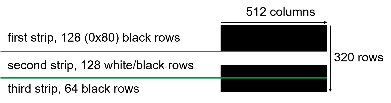
Let’s determine the strip sizes next: The first strip holds 128 rows, each of these rows holds 512 pixels (because ImageWidth = 512). Each pixel is represented by one bit (because we make a bilevel image). So the first strip contains 128 × 512 bits or (128 × 512) / 8 = 8192 bytes = 8 KiB. And isn’t that a coincidence, this aligns perfectly with the recommendation from the TIFF spec! The second strip has the same and the third strip half that size (because it contains only 64 rows). So we calculate the StripByteCounts values as 8192, 8192, and 4096 (or 2000, 2000, 1000 in hex).

As you see, this is the first time an IFD entry does not contain one single value but a list of values, so we have to set the count to 3 (the length of the list). The list values are stored as a consecutive sequence of length 3 (count) × 2 (size of a SHORT) = 6 bytes. Obviously that doesn’t fit into four bytes, so we need a pointer again. The same goes for StripOffsets which contains three (yet unknown) pointers of type SHORT. (Yes, that’s a pointer to a list of pointers …)

Tag  Type Count    Value
0116 0003 00000001 00800000                  # RowsPerStrip
0117 0003 00000003 ???????? → 2000 2000 1000 # StripByteCounts
0111 0003 00000003 ???????? → ???? ???? ???? # StripOffsets

And that’s it, we have put together all the IFD entries we need. Our Image File Directory is complete. Let’s review what we have so far:

## Image File Directory

Number of IFD entries.

    0008

Sequence of IFD entries (tag + type + count + value offset).

    0100 0003 00000001 02000000 # ImageWidth, 512 pixels
    0101 0003 00000001 01400000 # ImageLength, 320 pixels
    0106 0003 00000001 00000000 # PhotometricInterpretation, WhiteIsZero
    0111 0003 00000003 ???????? # StripOffsets, pointer
    0116 0003 00000001 00800000 # RowsPerStrip, 128
    0117 0003 00000003 ???????? # StripByteCounts, pointer
    011a 0005 00000001 ???????? # XResolution, pointer
    011b 0005 00000001 ???????? # YResolution, pointer

Offset of the next IFD or 0.

    00000000

Values referenced from the IFD that don’t fit into four bytes.

    ???? ???? ????    # StripOffsets, pointers
    2000 2000 1000    # StripByteCounts, 8/8/4 KiB
    0000012c 00000001 # XResolution, 300/1
    0000012c 00000001 # YResolution, 300/1

Note that we put the values referenced from the IFD right after the IFD itself. That’s certainly not the worst place for that data but it could just as well be almost anywhere else in the file. Yay pointers! And speaking of pointers …

Interlude: resolving pointers

You probably have noticed that we have accumulated quite a lot of placeholders where pointers should be. It’s about time we fix that.

As I said before, the use of offsets as pointers to locations in a file is common in binary file formats, and it’s in fact pretty simple (except that it’s easy to get lost counting but usually that’s not done manually, unless you’re writing binary by hand …). Again, an offset is simply a position in the file which is determined by counting bytes from the beginning of the file. The first byte has offset 0, and after that it’s just counting. Let’s see:

[Offset 0] ## Image File Header

Byte order (big endian) + number 42 + offset of first IFD.

    4d4d 002a 00000008 [8 bytes]

[Offset 8]

The file starts at offset 0, and that’s also where the Image File Header starts. (Note that we only count the bytes in the code blocks since that’s what will be in the resulting binary. We do not count the surrounding Markdown paragraphs, headlines, whitespace, line breaks, comments, etc.!) We know that the Image File Header holds 8 bytes, so after that we are at offset 8. That’s where the Image File Directory starts. The IFD begins with the number of entries (2 bytes), after that there are 8 12-byte entries, and then the 4-byte offset of the next IFD. So after the IFD we are at offset 8 + 2 + (8 × 12) + 4 = 110.

[Offset 8] ## Image File Directory

Number of IFD entries.

    0008                            [2 bytes]

Sequence of IFD entries (tag + type + count + value offset).

    0100 0003 00000001 02000000 ... [8 × 12 = 96 bytes]

Offset of the next IFD or 0.

    00000000                        [4 bytes]

[Offset 110]

Right after the IFD, at offset 110 (6e in hex) we put the values referenced from the IFD. These are the values some of the IFD entries point to, so these are the values whose offsets we need. Let’s count some more, and let’s switch to hex numbers while doing so because that’s what we will need anyway. (Many calculator applications can be switched to hex mode so it’s easy to add hex numbers without converting between hex and decimal all the time.)

Values referenced from the IFD that don’t fit into four bytes.

    [Offset 6e] ???? ???? ????    # StripOffsets    [6 bytes]
    [Offset 74] 2000 2000 1000    # StripByteCounts [6 bytes]
    [Offset 7a] 0000012c 00000001 # XResolution     [8 bytes]
    [Offset 82] 0000012c 00000001 # YResolution     [8 bytes]
    [Offset 8a]

And there we have the offsets! Now we just have to insert them into their respective IFD entries. For example, the XResolution value is stored at offset 7a, so that’s what we put into the XResolution IFD entry:

011a 0005 00000001 0000007a # XResolution, pointer

We can even resolve the pointers for the StripOffsets field. We haven’t created any image data yet, but we do know its structure, right? Remember we chose to arrange it into three strips of 8/8/4 KiB (or 2000/2000/1000 bytes, in hex). If we put the first strip just where we stopped counting offsets (i.e., right after the YResolution value) it starts at offset 8a. If we put the second strip right after the first and the third right after the second they in turn start at offsets 208a and 408a, respectively:

## Image Data

Three strips, containing 8/8/4 KiB of pixel data.

    [Offset 008a] ...
    [Offset 208a] ...
    [Offset 408a] ...

And that’s pretty much all there is to offsets and pointers. It’s tedious and error-prone, but at the end of the day it’s just counting and adding.

Image data

Finally, let’s create some image data. Remember, the first strip consists of 128 × 512 black pixels, so we need 128 × 512 1 bits, or 8192 (8 KiB) ff bytes. After that 4096 00 and 4096 ff bytes for the second, and then again 4096 ff bytes for the third strip. In principle, it’s easy:

## Image Data

Three strips, containing 8/8/4 KiB of pixel data.

    ff ff ff ...              # 8 KiB
    00 00 00 ... ff ff ff ... # 4 + 4 KiB
    ff ff ff ...              # 4 KiB

But obviously, it’s a bit painful to write these byte sequences by hand. So apart from the better readability and the possibility to add documentation and comments I hope you have come to appreciate already, here’s another advantage of Literate Binary over a plain hex editor: special hex syntax! Instead of typing ff bytes all day long (or resorting to programming to let the computer write it for you) you can just write this:

## Image Data

Three strips, containing 8/8/4 KiB of pixel data.

    (ff){8K}          # first strip, 128 black rows
    (00){4K} (ff){4K} # second strip, 64 white + 64 black rows
    (ff){4K}          # third strip, 64 black rows

If you are used to regular expressions this syntax may feel familiar, otherwise here’s a quick intro: (ff){8K} means “repeat the byte sequence ff 8K = 8 × 2¹⁰ = 8192 times” (the full syntax is documented here). That generates the expected image:

This and similar syntactic features of Literate Binary make writing some hex sequences, particularly repetitive and random patterns much easier. For example, repetitions can be nested (but just as with regular expressions, it takes a while to understand what’s happening here …):

(
  ((ff 00){32}){8} # one line of black/white squares
  ((00 ff){32}){8} # one line of white/black squares
){20}              # repeated 20 times

There’s also syntax for random data (. means “one random byte”) which is often useful if you have to generate some payload for a file but don’t really care what it is:

.{20K} # 20 KiB of random pixels

Epilogue

And that’s it, we have written a complete binary file by hand. For reference, here it is in its entirety (you can also find more or less the same file, but with much more documentation on GitHub):

# TIFF File Example

## Image File Header

Byte order (big endian) + number 42 + offset of first IFD.

    4d4d 002a 00000008

## Image File Directory

Number of IFD entries.

    0008

Sequence of IFD entries (tag + type + count + value offset).

    0100 0003 00000001 02000000 # ImageWidth
    0101 0003 00000001 01400000 # ImageLength
    0106 0003 00000001 00000000 # PhotometricInterpretation
    0111 0003 00000003 0000006e # StripOffsets, pointer
    0116 0003 00000001 00800000 # RowsPerStrip
    0117 0003 00000003 00000074 # StripByteCounts, pointer
    011a 0005 00000001 0000007a # XResolution, pointer
    011b 0005 00000001 00000082 # YResolution, pointer

Offset of the next IFD or 0.

    00000000

Values referenced from the IFD that don’t fit into four bytes.

    008a 208a 408a    # StripOffsets, pointers
    2000 2000 1000    # StripByteCounts, 8/8/4 KiB
    0000012c 00000001 # XResolution, 300/1
    0000012c 00000001 # YResolution, 300/1

## Image Data

Three strips, containing 8/8/4 KiB of pixel data.

    (ff){8K}          # first strip, 128 black rows
    (00){4K} (ff){4K} # second strip, 64 white + 64 black rows
    (ff){4K}          # third strip, 64 black rows

All that’s left now is turning the Markdown file into a proper binary. Get the lb tool, put it somewhere in your PATH (on Linux and MacOS you may also have to make it executable – hint: chmod u+x lb) and feed your Markdown file into it:

$ lb example.md --output example.tif

What’s next?

So you made it to the end of this post, congratulations! If you would like to play around some more on your own, here are some ideas for further tinkering:

Switch PhotometricInterpretation to 1 (BlackIsZero) and see what happens.
Read sections 4–6 of the TIFF spec to learn about grayscale and color images, building on the bilevel file we just created (it’s easy!).
Switch the byte order to little endian (rather boring, but maybe you learn something).
Find out about pad bytes and word boundaries (search the spec!).
Move things around in the file and adapt pointers.
Insert garbage (or hide data) between the regular file components.
Try to violate the specification and raise validation errors with JHOVE or other tools, then fix them. Examples:
- wrong order of IFD entries (see page 15)
- duplicate pointers (see page 26, example, another example)
- everything in Section 7: Additional Baseline TIFF Requirements (page 26)
Add example files or other information to the JHOVE wiki.
Read the specification of a different file format and write Literate Binary based on that.

Whatever you do, if you create something interesting (or funny) please consider sending me a pull request on GitHub to extend my collection of Literate Binary examples files!